large

A piece-wise additive model of survival data with non-linear rut

Omaku Peter Enesi1*, B. A. Oyejola2

1Department of Mathematics and Statistics, Federal Polytechnic, Nasarawa, Nigeria, 2Department of Statistics, University of Ilorin, Ilorin, Nigeria

Address for correspondence: Omaku Peter Enesi, Department of Mathematics and Statistics, Federal Polytechnic, Nasarawa, Nigeria. E-mail: omakupete@gmail.com
Submitted: 14-07-2020, Accepted: 18-07-2020, Published: 30-12-2020

ABSTRACT

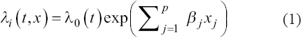
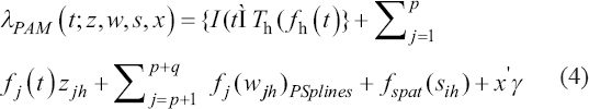
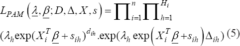
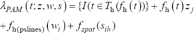
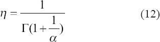
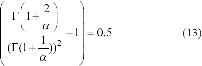
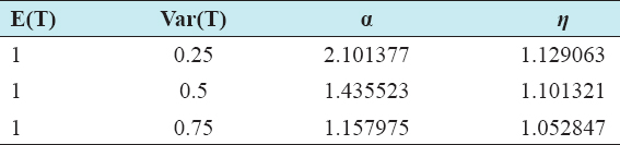
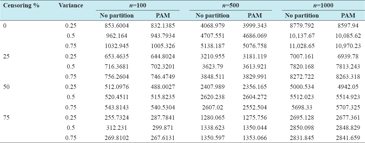
A critical step when developing multivariate risk prediction models is to decide which are the predictors that should be included and which ones could be neglected to get an accurate but interpretable model. The general additive models (GAMs) have come as quite an attractive procedure to handle covariate complexities in their various functional forms which is unlikely with the Cox model. In this study, a modification of piece-wise additive hazard model is proposed. Three levels of variance of Weibull distribution were assumed for baseline hazards in generating the data. The sensitivity of the baselines was accessed under four censoring percentages (0%, 25%, 50%, and 75%) and three sample sizes (n=100, 500, and 1000), for when models were single additive model (SAM) and when partitioned – piece wise additive model (PAM). A piece-wise Bayesian hazard model with structured additive predictors in which time-varying covariate and the functional form of continuous covariates were incorporated in a non-proportional hazards framework was developed. Hazard function was modeled through additive predictors that are capable of incorporating complex situations in a more flexible framework. Analysis was done utilizing MCMC simulation technique. Results revealed that the PAMs in most situations outperformed the SAMs with smaller DIC values and larger predictive powers with the log pseudo-marginal likelihood criterion.

Keywords: Continuous covariate functions, generalized additive model, penalty splines, piece-wise additive model, proportional hazard, single additive model, time-varying covariates


INTRODUCTION

In a ground breaking paper, Cox proposed a model for survival data in the proportional hazard frame work. Sir David Cox observed that if the proportional hazard assumption holds (or, is assumed to hold), then it is possible to estimate the effect of parameter(s) without any consideration of the hazard function.[1] Developing models in complex analysis may violate this assumption as the model may incorporate time-varying effects and covariates, thereby relaxing the proportional hazard assumption, and allowing the hazard ratio to depend on time t. A common approach to model time-varying effects is by piece-wise constant functions, as these are flexible enough to capture any shape of the baseline hazard or covariate effects,[2] for a frequentist and[3] and more recently[4] for a Bayesian approach.

The hazard model was further extended by Hennerfeind et al., Kneib and Fahrmeir,[5,6] to incorporate a flexible spatial generalization of the Cox model, a structured geo-additive predictor, including a spatial component for geographical effects and non-parametric terms for modeling unknown functional forms of the log-baseline hazard rate and non-linear effects of continuous covariates.

Generalized additive models (GAMs) are statistical models in which the conventional multiple linear regression is generalized to permit a much broader class of time-varying and non-linear functional form of continuous covariates and their effects, but still with additive relationships between response and predictor variables. GAMs, derived from the work of Hastie and Tibshirani,[7,8] provide flexible and effective means of moving out of the “linear rut”[9] in which a considerable amount of bio-statistical modeling is still located. Conventionally, non-linearity is handled through transformations and then estimation of linear models. Such an approach requires the researcher to have good knowledge of the correct functional form before the model is fitted when, in reality, the choice is very open and theory is usually vague. In contrast, the GAM represents an “adaptive” approach in which the data help guide the choice of appropriate functional form.[10]

In approaching these complexities in building a model, data are partitioned in bits of intervals and regularized estimation through penalized spline is carried out. The complexity of covariates included in models and the estimation method adopted by different authors such as Marano et al., Lang and Brezger[4,11] has, however, caught our attention in this study.

Motivated by this, we studied and compared the sensitivity of models under different censoring percentages, for several sample sizes within the framework of Weibull distributions whose shape and scale parameters are obtained by varying the variances while keeping the mean at 1; through the unit root function implemented in R.

The study further investigates: The performance of single additive models (SAMs) and the modified piece-wise additive extension or piece-wise additive models (PAMs) under various censoring percentages and sample sizes employing three levels Weibull baseline variance.

METHODOLOGY

The risk data used for this paper were simulated from a Weibull baseline hazard distribution which was used to generate survival times for sample sizes of 100, 500, and 1000, respectively. Various censoring levels or percentages of no censoring “0%,” low “about 25%,” moderate “about 50%,” and high “about 75%” were used.

Model Specification

The Cox hazard model

thumblarge

The baseline hazard rate is unspecified and assumes that covariates x=(x1,…,xp) act multiplicatively on the hazard rate through the exponential link function.[1]

Model Extension

thumblarge

Where, λi (t) is the hazard function for individual i at time t.

γ1 xi1γp xip: Are time invariant covariates.

γj xin (t): Time-dependent covariates

λ0 (t) is the baseline hazard function for an individual whose covariates x1xp all have values of 0.

An additive representation of model (1) is given by:

thumblarge

This is a reparameterization of the Cox model

Where, f0 (t)=logλ0 (t) is the functional form of the baseline hazard, which implies exp(f0 (t)). Other aspects of the model include the functions f1 (t) z1fp (t) zp which are the functional form of time-varying covariates z1,…,zp, the functions fj (w1)…fq (wq) are possibly non-linear effects of metrical covariates w1,…,wq and γ is the usual linear part of the predictor for some categorical covariates.[5,12]

Modification of Piece-wise Additive Models (PAMs)

The proposed model in bits of intervals is given as

thumblarge

with its various terms defined as:

The function fh=logλh is the baseline effect for the hth interval of PAM

The functions f1 (t) z11fp (t) zph are the functional form of time-varying covariates z11,…,zph in the hth interval, the functions fj (w11),…, fp (wqh) are possibly nonlinear effects of metrical covariates w1h,…,wqh in the hth interval, and fspat (sih) is a structured spatial effect, where s, s = 1, , S is either a spatial index, with s = si if subject i in the hth bit (interval) is from area s or it is an exact spatial coordinate s =(xi, ys), for example, for centroids of regions or if exact locations of individuals are known.

γ is the usual linear part of the predictor.

thumblarge

Where, for each subject i there is a product of Hi terms, Hi being the number of intervals in which the subject is followed. In the expression above, dih is the status of the ith subject within the interval Th (0 = alive or censored, 1 = failed); Dih is the time spent in Thby the subject. From expression (5), it may be seen that LPAM is proportional to the product of Poisson likelihoods for Dih with mean parameters:

thumblarge

. As a consequence, the expression of the Poisson regression model is:

thumblarge

Where, h(i) indicate the interval where ti falls, that is, the interval where individual i died or was censored,

αh = log(λh) are log-hazard parameters, and the term log(Dih) is an offset.

Bayesian P-splines Approach for Modeling the Unknown Functions

A number of competing approaches are available for modeling and estimating non-linear function fj of continuous covariates. These include smoothing splines,[8] local polynomials,[13] regression splines with adaptive knot selection,[14,15] and P-splines.[16,17] In this study, Bayesian version of penalized splines is employed following.[11] P-splines were introduced in a frequentist setting by Eilers and Marx, Marx and Eilers.[16,17] The basic idea of P-splines is to assume that an unknown smooth function fj (xj) of a continuous covariate xj can be approximated by a linear combination of B-spline basis functions Bm.[18] That is, denoting the m-th basis function by Bjm, we then obtain

thumblarge

The basic functions Bm are B-splines of degree l defined over a grid of equally spaced knots

thumblarge

, where s is the number of the equally spaced knots.

The Bayesian P-splines method is based on a hierarchical model with non-informative priors for the regression coefficients (b) and a Gaussian random walk (RW) prior of order d for the coefficients of the hazard function (B-spline), conditional to a smoothing parameter τ2 the general expression of the RW prior as suggested by Lang and Brezger, Kooperberg and Intrator[11,19] is the following:

thumblarge

The penalty matrix Kj is of the form Kj = DD, where D is a first or second order difference matrix.

For an independent and identical random effect, the penalty matrix is the identity matrix, that is, Kj=I. The variance parameter

thumblarge

controls the tradeoff between flexibility and smoothing and an inverse gamma prior (the conjugate prior) is assumed, that is,

thumblarge

.

Gaussian Random Field (GRF) Priors

For georeferenced data, it is commonly assumed that vi = v(si) arises from a Gaussian random field (GRF) {v(s),sϵS} such that v = (v1,…,vm) follows a multivariate Gaussian distribution as

thumblarge

, where τ2 measures the amount of spatial variation across locations and the (i, j) element of R is modeled as R[i, j] = ρ(si, sj). Here ρ(.,.) is a correlation function controlling the spatial dependence of v(s). In “survregbayes” package in R, the powered exponential correlation function

thumblarge

is used, where φ > 0 is a range parameter controlling the spatial decay over distance, vϵ (0,2] is a pre-specified shape parameter, and ‖ss’‖ refers to the distance (e.g., Euclidean, great-circle) between s and s’. Therefore, the prior GRF (τ2,∅) is defined as

thumblarge

i = 1,…, m where Pij is the (I, j) element of R–1[20]

Hazard Model with Regularized Functions

thumblarge

Where, B0 is the vector form of a B-spline of degree 0 defined for the follow-up period, and πβ and πτ2 are generic prior densities for the regression coefficients and the smoothing parameter.[20,21]

Regularized piece-wise additive model (RPAM)

thumblarge

The time-dependent effects for each covariate are:

thumblarge

; j = 1,…,p. Thus, for each Zj, its values are multiplied by a piece-wise constant function:

thumblarge

; in the parameters.

thumblarge

. This enables the effect of each Z1j to vary in each interval Th of the original partition of the follow-up:

thumblarge

for tTh. On the other hand, the effects of w1,…,wq have been represented through the general expression of B-splines, with the vector

thumblarge

including the spline basis of wi calculated for the ith individual. Thus, in this case, the degree and the knots of each spline are fixed following conventional rules. πβ and πτ2 are generic prior densities for the regression coefficients and the smoothing parameter.

Model Specification to Advance Simulation

Model 1:

thumblarge

Model 2:

thumblarge

Where, λPI is the hazard function when partitioning is ignored (PI) or SAM

Where, λPD is the hazard function when partitioning is done (PD) or piece wise additive model (PAM).

Test for Non-proportionality

To test the hypothesis that the proportional hazard assumption is valid, the following statement of hypothesis is made.

H0: δ1=δ2=⋯=δp (Assumption is valid)

H1: At least one of the δis is not equal to zero (Assumption violated)

Decision rule: Reject H0 if Pα (level of significance)

Residual measures are used to investigate the departure from the proportional hazard assumption. Schoenfeld residuals are used to test the assumption of proportionality. Schoenfeld residuals are usually calculated at every failure of time under the proportional hazard assumption and usually not defined for censored observations. The overall significance test is called the global test of the model, sighted in Adeniyi and Akinrefon.[22]

Data Analysis

The data are simulated using the functional form of time-varying covariate by Bender et al.[23] given as

thumblarge

The functional form of the continuous covariates as in Brezger[24] is given as:

thumblarge

where xi~U(–3,3).

For spatial frailty, we propose, S = pnorm(v) and v~mvrnorm(1,S); if S=pnorm(v) then S~mvrnorm, where, S is the covariance matrix for spatial correlation.

Coordinates for spatial correlations follow the uniform distribution. s1 = runif(N,0,40) and s2 = runif(N,0,100),[25] obtained the shape and scale parameters of the Weibull distribution from the following

thumblarge

And

thumblarge

for a convenience choice of mean 1 and variance 0.5. Using the uniroot function in R. Parameters were given to be approximately α=1.435523 and η=1.101321. We considered studying the impact of increasing and decreasing the variance of the Weibull distribution while keeping the mean at 1. The result is displayed in Table 1.

Table 1: Shape and scale parameters of the Weibull distributions

thumblarge

Data simulation and analysis were carried out in R using the coda package for spBayesSurv, version 3.6.2. Comparisons were done using deviance information criterion (DIC) (smaller is better) which places emphasis on the relative quality of model fitting and log pseudo-marginal likelihood (LPML) (larger is better) focuses on the predictive performance. Both criteria are readily computed from the MCMC output.

RESULTS

Interpretation

From Tables 2 and 3: The PAMs perform better than the SAMs – by Hennerfeind et al., and Abiodun.[5,12] This suggests that smoothening with smaller bit of intervals is better than when partitioning is ignored. It was observed that P-spline smoothing for continuous covariates in smaller sample sizes is better than in larger sizes. Increments in variance parameter for the baseline distribution reduce the precision and predictive power of the models (high values of DIC and low values of LPML). This was particularly observed in PAMs for intermediate and high levels of Weibull baseline variance at 75% censoring when sample size is n = 500 and 1000, and for intermediate levels of variance at 50% and 75% censoring, when n = 1000.

thumblarge

Table 2: DIC values for levels of censoring, three levels of Weibull baseline variance and sample sizes for partitioned and no partition models

Table 3: LPML values for levels of censoring, three levels of Weibull baseline variance, and sample sizes for partitioned and no partition models

thumblarge

Precision and predictive power (based on DIC and LPML) improved with increase in censoring percentages. PAM outperformed the SAMs for reduced amount of the spread of event times and censoring percentages. Increase in sample size induces increase in DIC and a decrease in LPML values.

In general when dealing with survival analysis data in a non-proportional framework, with complexities associated with covariate combinations, smaller sample sizes produce a better model representation for SAMs and much better when the models are represented within bits of intervals in constant hazards – PAMs. Increase in the variability in the baseline distribution seems to increase the spread of survival times which further reduces model precision.

CONCLUSION

This research brings to knowledge the essence of performing survival data analysis in bits of time, especially in scenarios with covariate complexities, which makes interpretation of hazard rates difficult. PAM has been shown in this study to be better than SAM at all levels of variance, censoring percentages, and sample sizes.

REFERENCES

1.  Abiodun AA. Analyzing competing risk survival time data using cox and parametric proportional hazards models. JNSA 2007;19:74-9.

2.  Verweij PJ, van Houwelingen HC. Time-dependent effects of fixed covariates in cox regression. Royal Stat Soc Series B 1995;34:187-220.

3.  Gamerman D. Bayes estimation of the piece-wise exponential distribution. IEEE Trans Reliab1994;43:128-31.

4.  Marano G, Boracchi P, Biganzoli EM. Estimation of the piecewise exponential model by Bayesian P-splines via Gibbs sampling:Robustness and reliability of posterior estimates. Open J Stat 2016;6:451-68.

5.  Hennerfeind A, Brezger A, Fahrmeir L. Geoadditive survival models. J Am Stat Assoc 2006;101:1065-75.

6.  Kneib T, Fahrmeir L. A mixed model approach for geo additive hazard regression. Scand J Stat 2007;34:207-28.

7.  Hastie T, Tibshirani R. Genemlized additive models. Stat Sdolce 1986;1:297-318

8.  Hastie T, Tibshirani R. Generalized Additive Models. London:Chapman and Hall;1990.

9.  Jones K, Almond S. Moving out of the linear rut the possibilities of generalized additive models. Trans Inst Br Geogr 1992;17:434-47.

10.  Marra G, Wood SN. Practical variable selection for generalized additive models. Comput Stat Data Anal 2011;55:2372-87.

11.  Lang S, Brezger A. Bayesian P-splines. J Comput Graphical Stat 2004;13:183-212.

12.  Abiodun AA. A Bayesian approach to exploring unobserved heterogeneity in clustered survival and competing risk data. JNSA 2009;20:1-13.

13.  Fan J, Gijbels I. Local Polynomial Modelling and its Applications. London:Chapman and Hall;1996.

14.  Friedman J, Silverman B. Flexible parsimonious smoothing and additive modelling (with discussion). Technometrics 1989;31:3-39.

15.  Stone C, Hamsen M, Kooperberg C, Truong Y. Polynomial splines and their tensor products in extended linear modelling. Ann Stat 1997;25:1371-470.

16.  Eilers PH, Marx BD. Flexible smoothing using B-splines and penalized likelihood (with comments and rejoinder). Stat Sci 1996;11:89-121.

17.  Marx DB, Eilers HC. Direct generalized additive modelling with penalized likelihood. Comput Stat Data Anal 1998;26:93-209.

18.  De Boor C. A Practical Guide to Splines. New York:Springer-Verlag;1978.

19.  Kooperberg C, Intrator N. Trees and splines in survival analysis. Stat Methods Med Res 1995;4:237-61.

20.  Zhou H, Hanson T. A unified framework for fitting bayesian semiparametric models to arbitrarily censored survival data, including spatially-referenced data. J Am Stat Assoc 2017;113:571-81.

21.  Omaku PE, Ibinayin JS, Tanko N, Braimah JO. A modified additive hazard model for some risk factors associated with hypertensive condition. AJMS 2020;3:1-8.

22.  Adeniyi OI, Akinrefon AA. First birth interval:Cox regression model with time varying covariates. CJPL 2018;6:1-7.

23.  Bender R, Augustin T, Blettner M. Generating survival times to simulate cox proportional hazards models. Stat Med 2005;24:1713-23.

24.  Brezger A. Bayesian P-splines in Structured Additive Regression Models. PhD Thesis. Munich:Springer-Verlag, LMU;2004.

25.  Ulviya A. Frailty Models for Modelling Heterogeneity. Canada:McMasters University;2013.